EEL6825: HW#4

Due Wednesday, November 8, 2000 in class. This is your final homework assignment. Late homework will lose 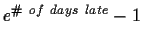$e^{\char93 ~of~days~late} -1$ percentage points. To see the current late penalty, click http://www.cnel.ufl.edu/analog/harris/latepoints.html

Also, note that Exam 2 has been bushed back one week to Monday, November 13, same time, room TBA.

PART A: Textbook Problems Answer the following questions, you should not use a computer.

A1

(5 points)

Class $\omega_1$ points are:

$$\left[ \begin{array}{c} -1 \\ -1 \\ +1 \end{array}\right] \... ...t] \left[ \begin{array}{c} +1 \\ -1 \\ -1 \end{array}\right]$$

Class $\omega_2$ points are:

$$\left[ \begin{array}{c} +1 \\ +1 \\ -1 \end{array}\right] \... ...t] \left[ \begin{array}{c} -1 \\ +1 \\ +1 \end{array}\right]$$

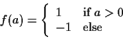
Find any weight vector w such that w^Tx>0 for all class $\omega_1$ points and w^Tx<0 for all class $\omega_2$ points. Justify your answer.

A2

(5 points) The density function of a two-dimensional random vector x consists of four impulses at (0,3) (0,1) (1,0) and (3,0) with probability of 1/4 for each. Find the K-L expansion. Compute the mean-square error when one feature is eliminated. Compute the contribution of each point to the mean-square error.

A3

(5 points) In one paragraph, compare the three types of classifiers we have discussed in the class (parametric, nonparametric and neural networks). Contrast them in terms of training time, testing time, and the number of data points required.

PART B: KL and Continuous Distribution

You are given two three-dimensional normal distributions with the following means and covariance matrices:

$\mu_1= \left[ \begin{array}{c} -1 \\ 1 \\ 0 \end{array}\right]$ $\mu_2= \left[ \begin{array}{c} 1 \\ -1 \\ 0 \end{array}\right]$ $\Sigma_1= \left[ \begin{array}{ccc} 1&0&0 \\ 0&1&0 \\ 0&0&0 \end{array}\right]$ $\Sigma_2= \left[ \begin{array}{ccc} 5&2&0 \\ 2&1&0 \\ 0&0&0 \end{array}\right]$

Assume that $P(\omega_1)=P(\omega_2)=1/2$ Answer the following questions relating to using the K-L transform for dimensionality reduction.

B1

(5 points) Compute the combined mean ($\mu$) and covariance matrix ($\Sigma$) for the data in this problem. Hint: Remember that the combined distribution of two equally likely normal distributions is not a normal distribution but the combined covariance matrix can be expressed as:

$$\Sigma = \frac{\Sigma_1 + \Sigma_2}{2} + (\frac{\mu_1-\mu_2}{2})(\frac{\mu_1-\mu_2}{2})^T$$

B2

(5 points) Compute all of the eigenvalues and eigenvectors of $\Sigma$.

B3

(5 points) If you had to drop one linear feature, which eigenvalue direction would you drop? Comment on the likely resulting change (if any) in the error for representation and for classification.

B4

(5 points) If you had to drop two linear features, which two eigenvalue directions would you drop? Comment on the likely resulting change (if any) in the error for representation and for classification.

B5

(5 points) Draw a very rough sketch 2-D sketch of the two distributions and show the key linear features under consideration. You do not have to draw exact equiprobability contours for each distribution. Make clear which direction you are deciding to keep (from your answer to part B4).

PART C: Neural Networks

Consider the following sample points: The samples from class 1 are: $\left[ \begin{array}{c} 1 \\ 1 \end{array} \right] \left[ \begin{array}{c} 1 \... ... \\ 1 \end{array} \right] \left[ \begin{array}{c} -1 \\ -1 \end{array} \right]$The samples from class 2 are: $\left[ \begin{array}{c} 0 \\ 2 \end{array} \right] \left[ \begin{array}{c} 2 \... ...2 \\ 0 \end{array} \right] \left[ \begin{array}{c} 0 \\ -2 \end{array} \right]$

Answer the following questions regarding the neural network solution to this problem.

C1

(5 points) How many hidden nodes are required to solve this problem? Explain.

C2

(5 points) Assume the sigmoid activation function of the neural network to be:

$$f(a) = \left\{ \begin{array}{ll} 1 & \mbox{if $a>0$} \\ -1 & \mbox{else} \end{array} \right.$$

Derive a neural network architecture that solves this problem. The final output of your neural network should be +1 for class 1 and -1 for class 2. Provide all of the necessary weight values for architecture with the minimum number of hidden units. Explain your reasoning and justify your results.

C3

(5 points) The hard limiting step function in [C2] is not used in practice. Explain why not.

C4

(50 points) Run a backpropagation algorithm to solve this problem. You are strongly recommended to use the matlab neural network toolbox that was discussed in class but you are free to use whatever software you like or even to program your own. Use the same architecture that you came up with in [C2] only with a different sigmoid. Show a few plots of MSE vs. epoch.

C5

(5 points) Hand in a plot of the decision boundaries for class 1 and class 2 along with the data points. There should be no errors. Note: it may be helpful for you to periodically plot these regions as the algorithm is running to see how far you are away from the correct solution.

As usual, include all plots and answers to questions in the first part of your document. All matlab code that you write should be included in the second part.